ATOR (Arc-Team Open Research).
The blog spreads tests, problems and results of Arc-Team research in archaeology, following the guidelines of the OpArc (Open Archaeology) project.
In the last weeks we started again with the development of ArcheOS 5 (codename Theodoric) and I have to say that the first results are really promising, especially thanks to the work of Fabrizio Furnari and Romain Janvier.
The reorganization of the whole system, planned by Fabrizio, is leading to a better management of the entire project. Moreover the division of the internal software in thematic metapackages (CAD, GIS, etc...) will help final users in customizing their own version of ArcheOS (in accordance with their specific needs).
On the other hand, Romain is working really hard to build source packages of the different applications, so that ArcheOS 5 will be architecture independent.
Last but not least, the 3D artist Cicero Moraes is preparing a brand new artwork for the upcoming release. If you are curious, just take a look on the preview for the splashscreen below.
New artwork from Cicero Moraes
So, what's missing now? Just you!
We need your help to improve ArcheOS 5!
We want you, and GNU ;)
Any kind of help is welcome! Some examples? You can give us suggestions for a better software selection, or write tutorial (as well as record videotutorial). If you have some computer skills, you can package the missing applications, or develop new ones...
In any case, you can find us as usual on the developer mailing list or, even better, in our brand new IRC chanel (thanks to Fabrizio). The server is FreeNode and the channel #archeos.
I prepared a short videotutorial to illustrate how to join our channel in a fast way.
manageR is a QGIS plugin
providing a simple and usefull interface to R statistical
programming environment (http://www.r-project.org/).
It is created by Carson J. Q. Farmer (http://www.ftools.ca/manageR)
and is downloadable from this repository:
http://www.ftools.ca/cfarmerQgisRepo.xml.
To install it in QGIS is enough
add such repository in QGIS
Python Plugin Installer
(Plugins → Fetch Python Plugins).
One of the most interesting things is
that you can take data directly from the .dbf table of the shapefile
layer loaded in QGIS and process them in R environment. Usually, when
I work with PostgreSQL/PostGIS or SQLite/SpatiaLite for managing
attributes table of vector layers, I connect directly database with R
using RODBC or RSQLite packages. But if I have to use shapefiles and
their .dbf tables, manageR could be a good solution, specially
for fast and simple works.
Here, I would like to present a small
example of plugin's use. In QGIS I created a distribution map of
Roman funerary sites in Trentino-Alto Adige region (Northern Italy).
The sites (blue dots) are registered in a simple shapefile and every
single point is associated to a record stored in a .dbf table. As
usual, the .dbf table is divided in several columns each of which
contains different attributes about sites (ID, coordinates, height,
date, etc.).
I need to plot an histogram of heights
above sea level to get an immediate view of sites distribution based
on heights. I can launch manageR from QGIS.
At first sight, manageR
is a simple GUI that includes R command line, some toolbars for
managing data, graphic devices, history, etc. and several buttons to
make some of the most common statistical analysis.
As I said, in manageR I can
import layer attributes with button “Action → Import Layers
Attribute” (or CTRL+T) and then I can select the column I need
(in my case, “height”) using R language.
Typing in R command line or using
button “Analysis” in main toolbar, I can select and launch
the statistical function I need and plot the diagram; in my example I
plotted an histogram of heights a.s.l. of my funerary sites.
This is a simple example, but manageR
plugin could be a very usefull tool for archaeologists, also for more
complex works. Its main advantage is that it works directly with .dbf
table, avoiding the export of data or the opening of .dbf file in
Calc/Excel.
The Australopithecus afarensis was an hominid that lived between 4 and 2 millions of years past.
They had biped behavior and the appearence of apes.
In this post I'll talk about my little adventure to reconstruct the face of this specie.
This work is a type of continuation of Taung Project, because the knowledge used there was tapped here, with some increase of the technic.
I have to thank to Moacir Elias Santos, a Brazilian archaeologist that took a serie of pictures of a cast skull on Museu Egipcio e Rosacruz.
The skull used was reconstructed with PPT GUI (scanning by picture).
To increase the quality of the reconstruction, I used a CT-Scan of a chimpanzee.
The skull of chimp was deformed using Lattice modifier on Blender 3D, until match with the Australopithecus skull. Obviously, the skin was deformed too.
After this, I used the reference of the deformed skin to modeling the final face.
The following steps were the same explained in other posts.
This post is about a practical application of a serie of studies published here in this blog.
After I started to study about forensic facial reconstruction I saw that is much more easy to find videos of CT-Scan than the DICOM files and other tomography formats.
A way to convert a video in a reconstructed mesh was described here.
Some days ago I was reading about mummies (desperate to find a CT-Scan) and I found this post:
It talks about a child mummy of St. Louis, that lived in a range of 40 BC and 130 AD. He died with 7 or 8 months.
Inside the matter had a video with some seconds of a CT-Scan slicing. I was able to convert it in a reconstructed mesh, and after I found a video on Youtbe with more qualty and I used it to make the final mesh, used in this post.
I downloaded the video with Videodownload Helper (Firefox) and it was converted in a image sequence and after in a serie of DICOM files.
Unfortunately I lost the original vetorial file and now we have only the infographic in Portuguese version, like you can see below (but it have a lot of images, that dispensing you to read it).
To make a reconstruction with historical and archaeological foundation I had the help of Moacir Elias Santos, archaeologist of the Egypt Museum and Rosacruz, from Brazil.
The animated gif above shows the extracted frames of the animation converted into a CT-Scan. I reduced the slices to make it more didatic.
I had a serie of dificulties to find landmarks to use on the child's face, cause appear that it doesn't exist. So I use a average of 3-8 year and rescale it to have at least a reference.
I use a serie of babies pictures to draw the line of the neck and ears.
Moacir sent me a compose image with the original mummy, that you can see below.
I hope you enjoy this post. I see you in the next. A big hug!
One of the main problem in doing videotutorials for ArcheOS 4 (Caesar) regarded the possibility to record the desktop activities when using 3D applications. Here is my report about this topic in ArcheOS ML. As you can read, the software we chose (recordMyDesktop) was not able to record videos (just a series of screenshots) of windows displaying 3D objects (like other similar tools: Istanbul, Xvidcap, Shuter).
Since I was using ArcheOS Caesar, I solved the problem with glc, before, and with ffmpeg, later (thanks to this post of Cicero Moraes). These two options have certainly high performance, but they are not user friendly for newbies.
Now that we started again with the development of ArcheOS 5, I think we will need a simple tool to record video of 3D applications and maybe I found a good solution: Vokoscreen.
The video below shows a fast test I did with this software. The data comes from the Taung Project and were developed by Cicero Moraes.
With this new tool I hope that ArcheOS users will help us in doing videotutorials or simply in recording demonstrative videos of Theodoric in action.
Rolf R Bakke Multicopter from HobbyKing (work in progress)
we bought a NAZA dji. It is not a Open Hardware project, but a low cost solution to obtain aerial pictures. This drone has a perfect implementation of the GPS module and a revolutionary way of flight; it offers three types of control modes:
Manual (M) = manual free flight
Attitude (A) = free flight with altitude lock and high attitude stabilize
GPS = free flight with hold final position
The movie below show how the GPS works to hold the position till the remote control gives new moving command.
We didn't try yet the RTH (Return To Home); as soon as possible i will upload a new movie about it.
More than ever before 3D models have become a "physical" part of our life, how we can see in the internet with 3D services of printing.
Some people have many difficult to get a model to print... well, not only to print, but to write an scientific article, make a job, or just have fun.
With this tutorial you'll learn how to scan 3D objects to use it the way you want.
Before all, I would like to thank all friends that help me to write this tutorial mainly Bob Max of the ExporttoCanoma's blog that publish interesting posts about GIS and now are interested in SfM (like all good nerd who works with 3D).
It's impossible to forget Pierre Moulon, the developer os Python Photogrammetry Toolbox (PPT), and Luca Bezzi e Alessandro Bezzi, developers of the ArcheOS and PPT GUI.
This tutorial includes many examples and some source files that will help you to learn how works the PPT.
So, lets go!
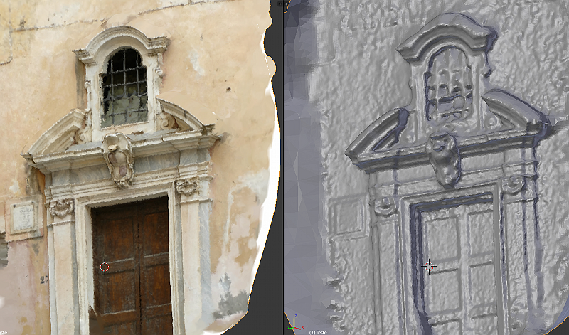
The image above show the object that we'll scan in this tutorial
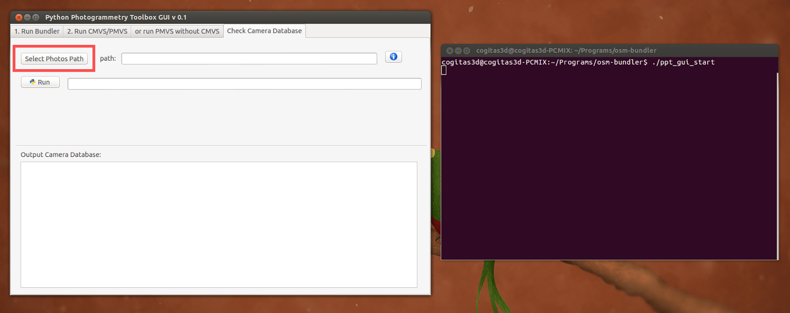
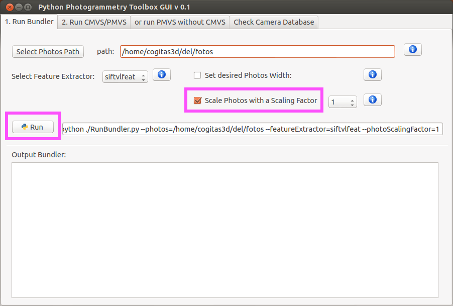
1) To make a good scan quality, click on “Scale Photos with a Scaling Factor”, by default, the value will be 1. If you have a computer with less power of processing, do not make this step (1), and go directly for the step bellow (2).
2) Click on “Run”.
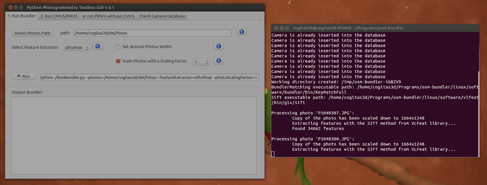
Wait a few minutes, the program will solve the point clouds.
You will know that the solve is done when in the Terminal appear the message:
Finished! See the results in the '/tmp/DIRECTORY' directory
In this case the message was: Finished! See the results in the '/tmp/osm-bundler-ibBZV9' directory
The Nautilus will be opened to, showing the directory with the files.
OBS.: If you area really curious, you can open the Bundle directory and see the .PLY files in Meshlab. But is better wait, because this point clouds is not good to make reconstruction/convertion into a mesh.
Go to the Terminal, where appeared the path with the solve, and make a copy of it.
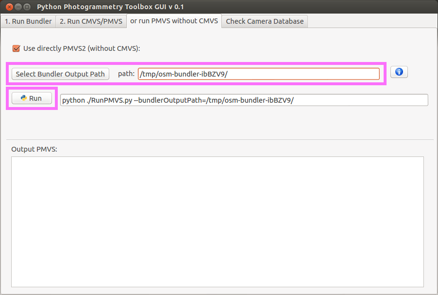
1) Go to the “or run PMVS without CMVS” 2) Click in “Use directly PMVS2 (without CMVS)”
1) Paste the path in “Select Bundler Output Path” 2) Click on “Run
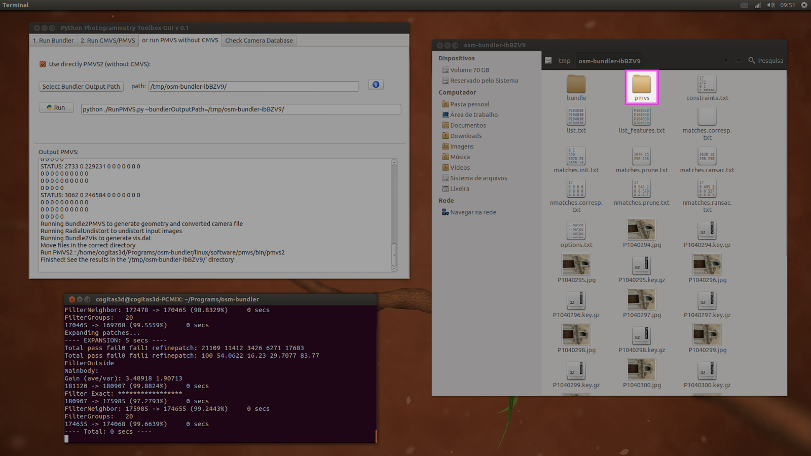
When the process is done, you’ll see a new directory named “pmvs” appear.
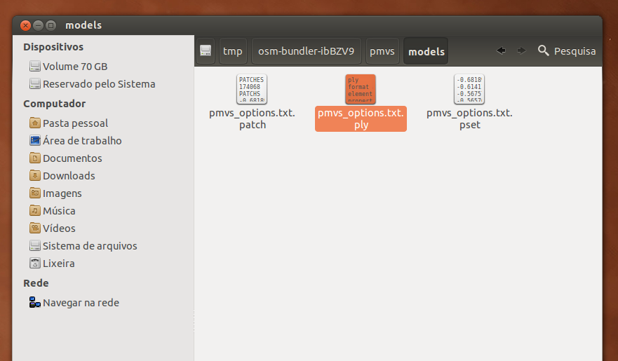
So, you have to enter in “models” and search for a file named “pmvs_options.txt.ply”. If all is OK it is the final process of solving.
OBS.: It’s a good idea copy the osm-* directory for your home, because it will be lost in the next boot, because the /tmp directory.
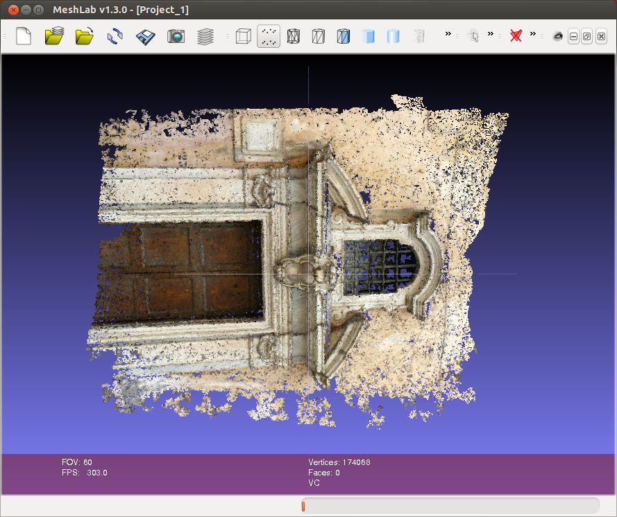
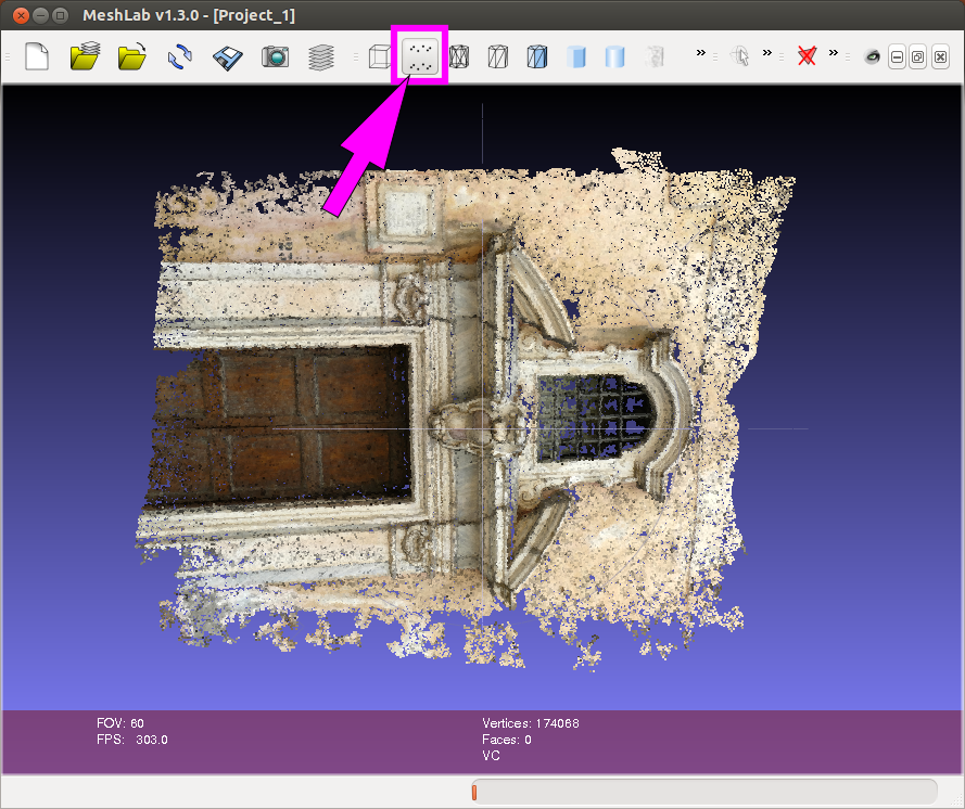
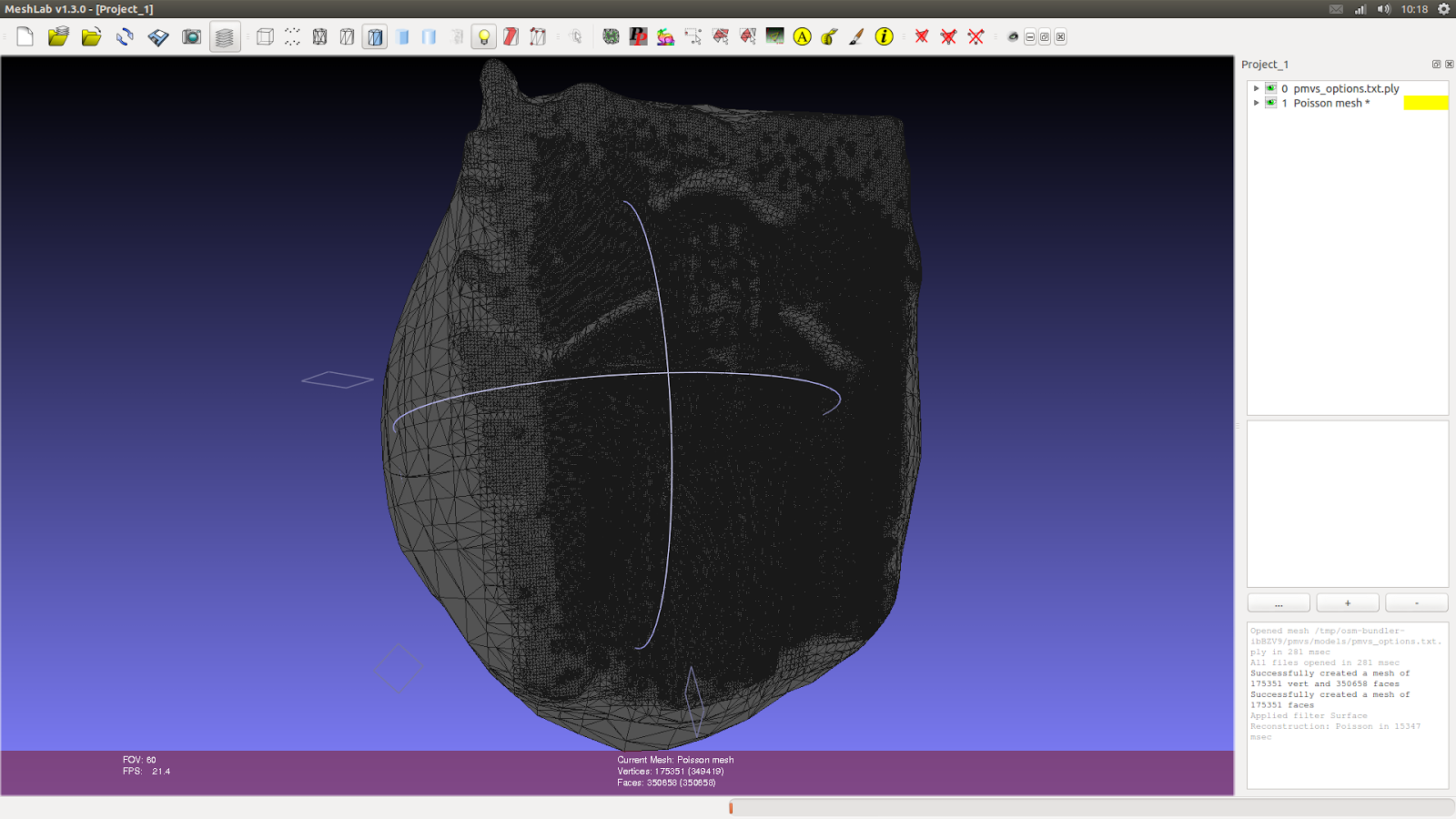
When you open the “pmvs_options.txt.ply” file in Meshlab you’ll see that the points cloud is really dense now, with almost the quality of a picture.
Only appear a picture or a mesh... notice that the “Points” is a way of view selected.
If you select “Flat Lines” for an exemple, the points clouds will desappear... because, obviously... it’s a --points-- cloud.
Click again in “Points” to see the points cloud and:
1) Click on “Show Layer Dialog” (A)
2) So, will appear a new element in the interface with the name of the object, in this case “pmvs_options.txt.ply” (B)
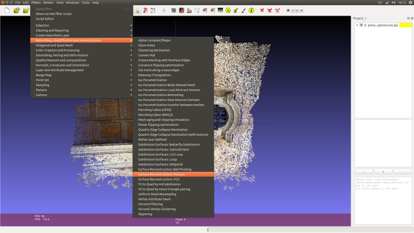
Go to “Filters” -> “Remeshing, simplification and reconstruction” -> “Surface Reconstruction: Poisson”
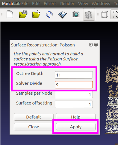
A new window will appear with the defaults value of “Octree Depth” and “Solver Divide”
1) Change the values to:
Octree Depth: 11
Solver Divide: 9
2) Click in “Apply”
OBS: This vlues can crash the program if you computer do not have a good power of processing.
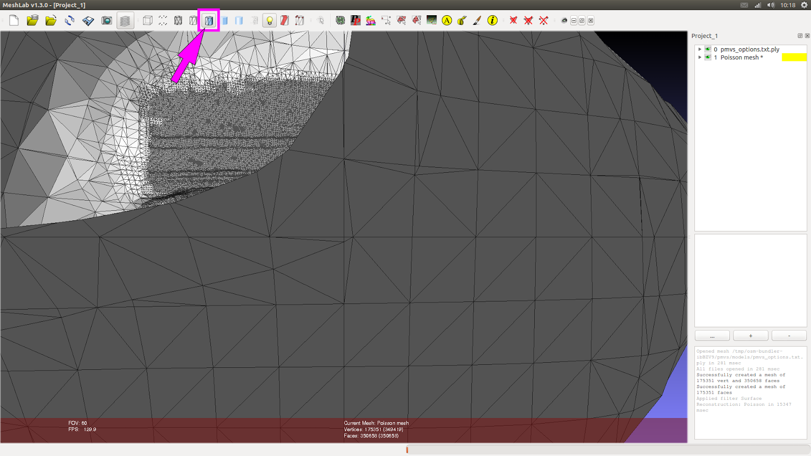
If all runs OK, you will notice two things:
1) A lot of new write points over the reconstruction.
2) A new layer in the upper right named “1 Poisson mesh *”
But, when we comeback to “Flat Line” to see the mesh, strange things can happen. In this case, the algotithm Poison created one type of ball to reconstruct the mesh.
We can see it better when we orbit away the model.
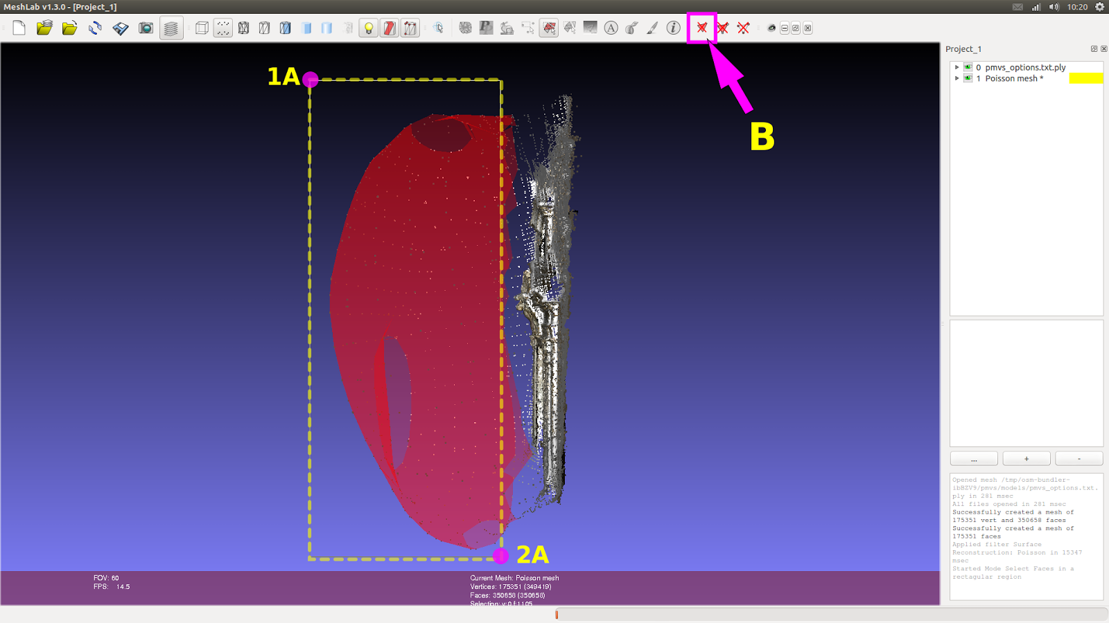
So, to make the door visible, we:
1) Come back to the “Points” view (A)
2) Orbit the scene to see the side of the door.
3) Click on “Select faces in a rectangular region”
So:
1) We make a window selection on the region that will be deleted (1A-2A)
2) Click on “Delete the current set of selected faces”.
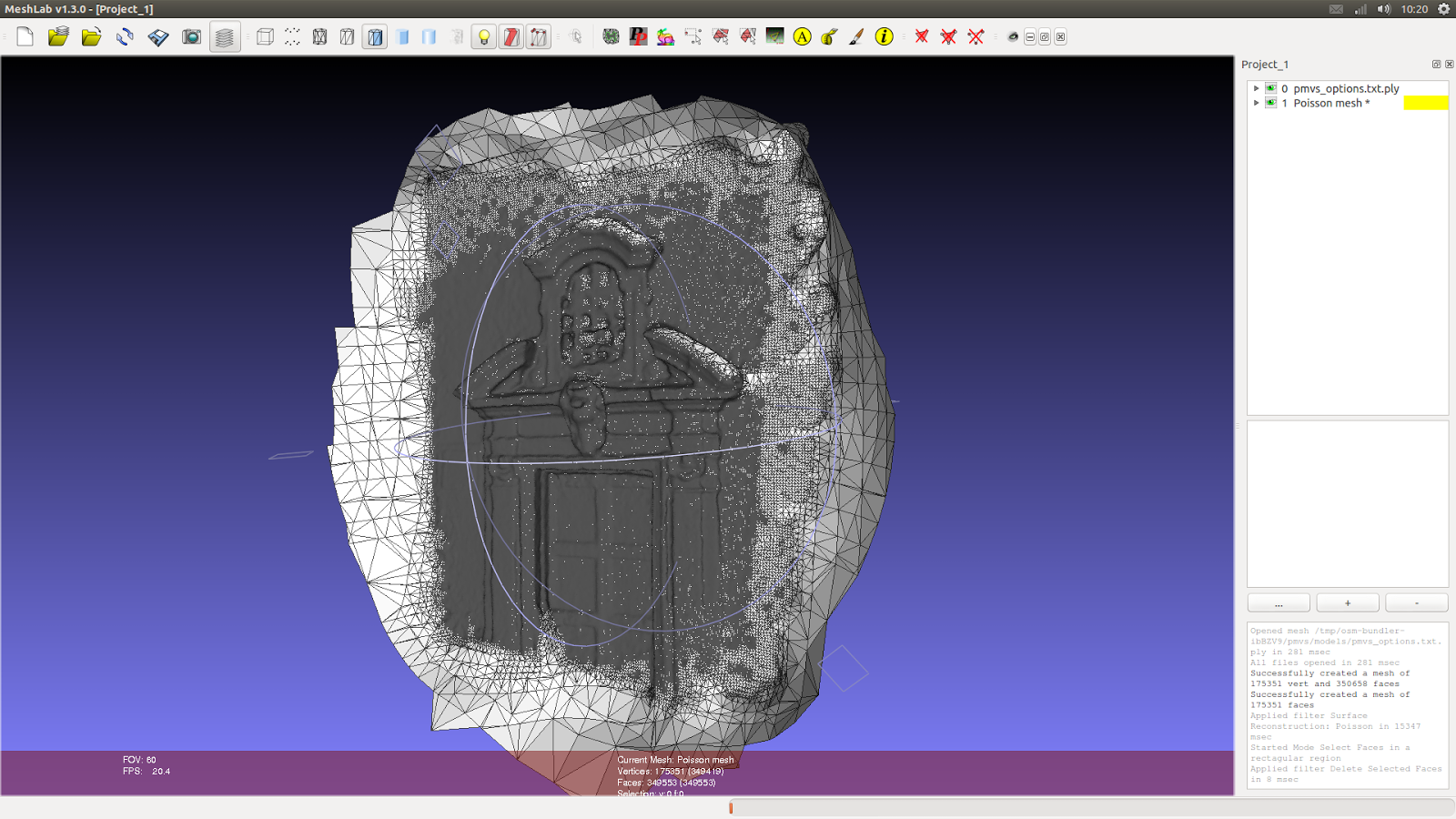
Now we can see the mesh in the correct side.
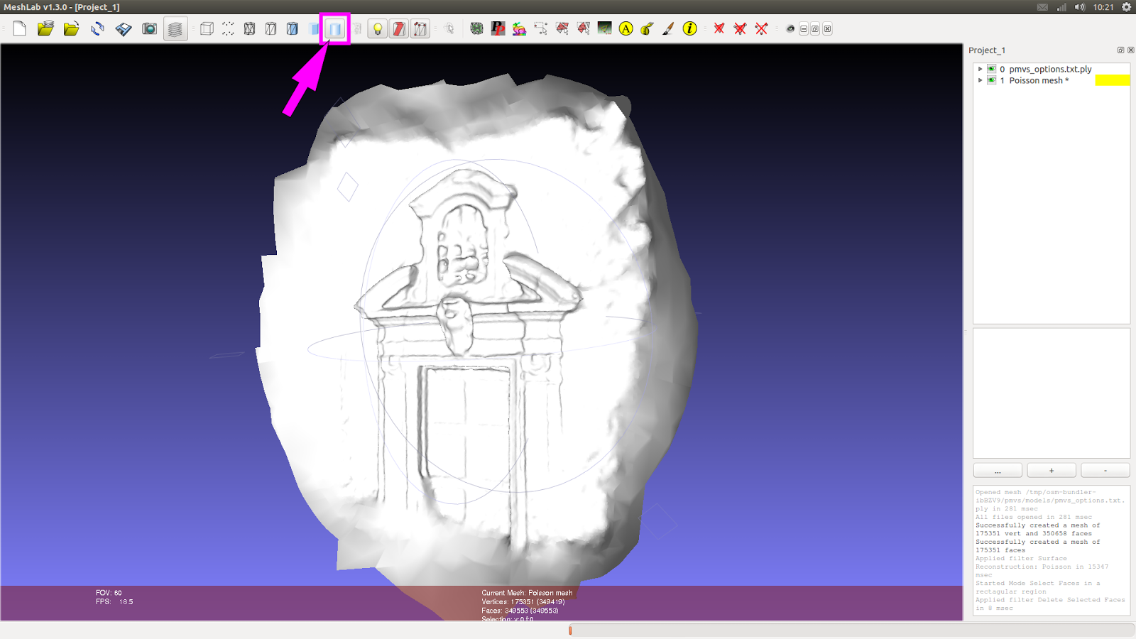
But, when we change the type of view to “Smooth”, we see the mesh write without the colors of the points cloud.
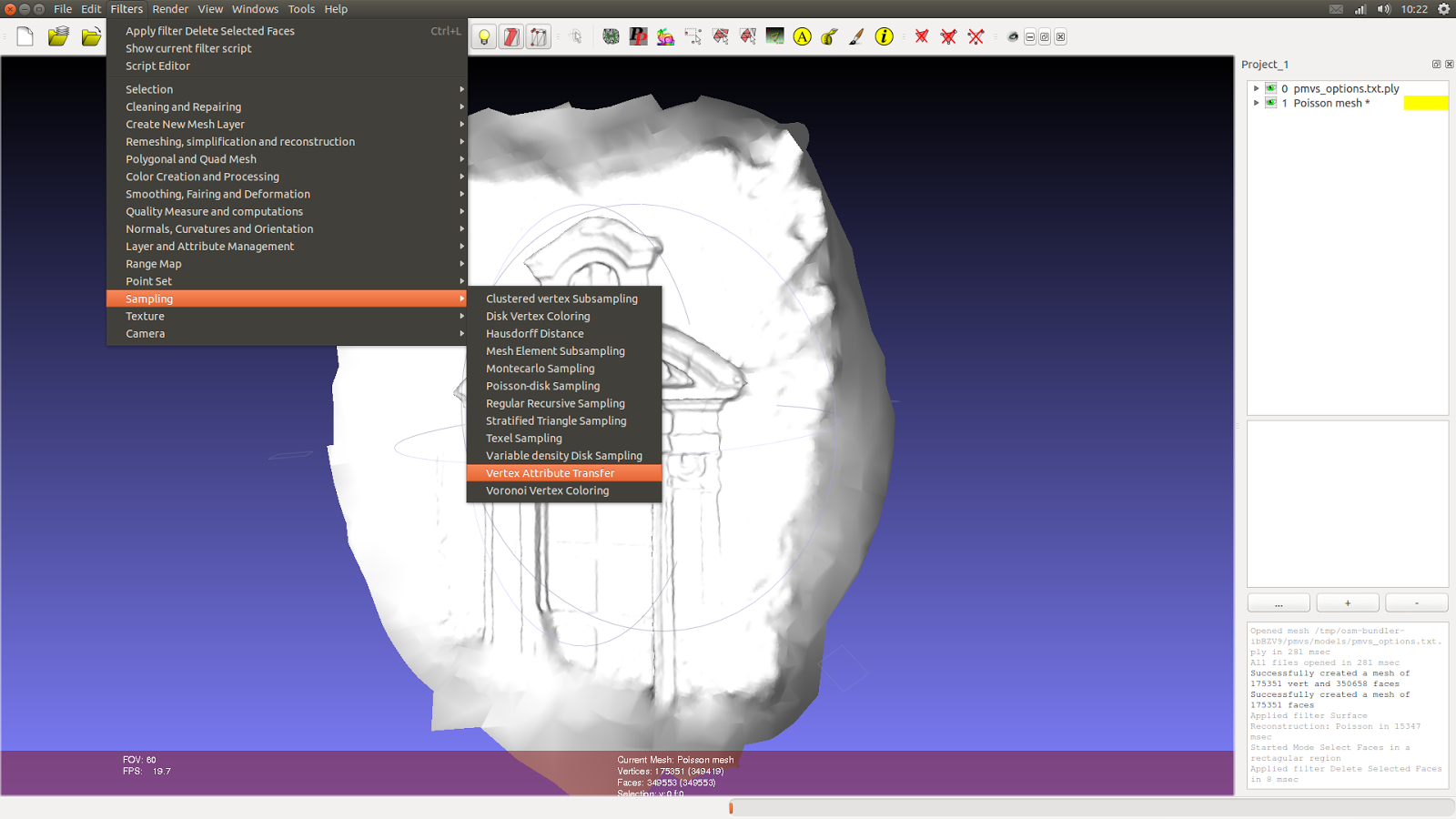
To paint the mesh with the color of the points cloud we can go to:
Filters -> Sampling -> Vertex Attribute Transfer
A substancial part of this step was learned with this video: http://vimeo.com/14783202
A new window will appear.
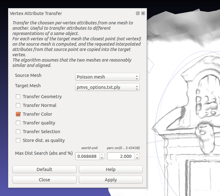
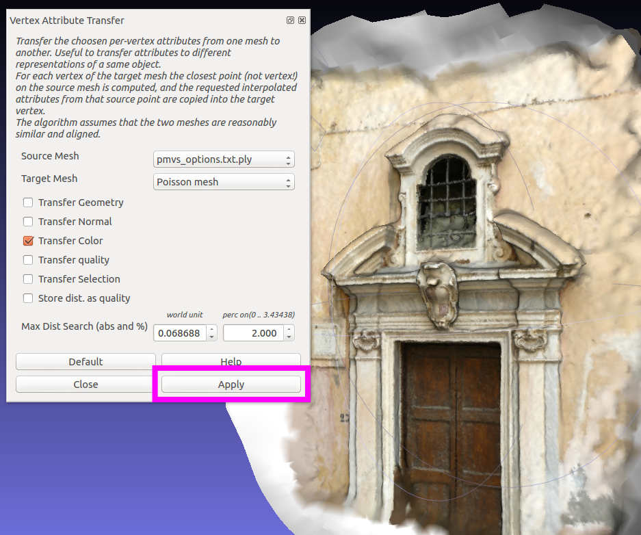
You’ll have to invert the objects, because the “pmvs_options.txt.ply” is the real source mesh, that will be the base to paint, and the “Poisson mesh” will receibe the colors, so it is the Target mesh.
When you click on “Apply” immediatly you’ll see the mesh colored, like the image above.
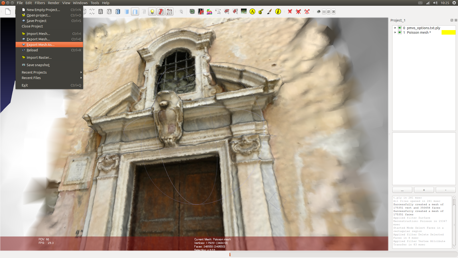
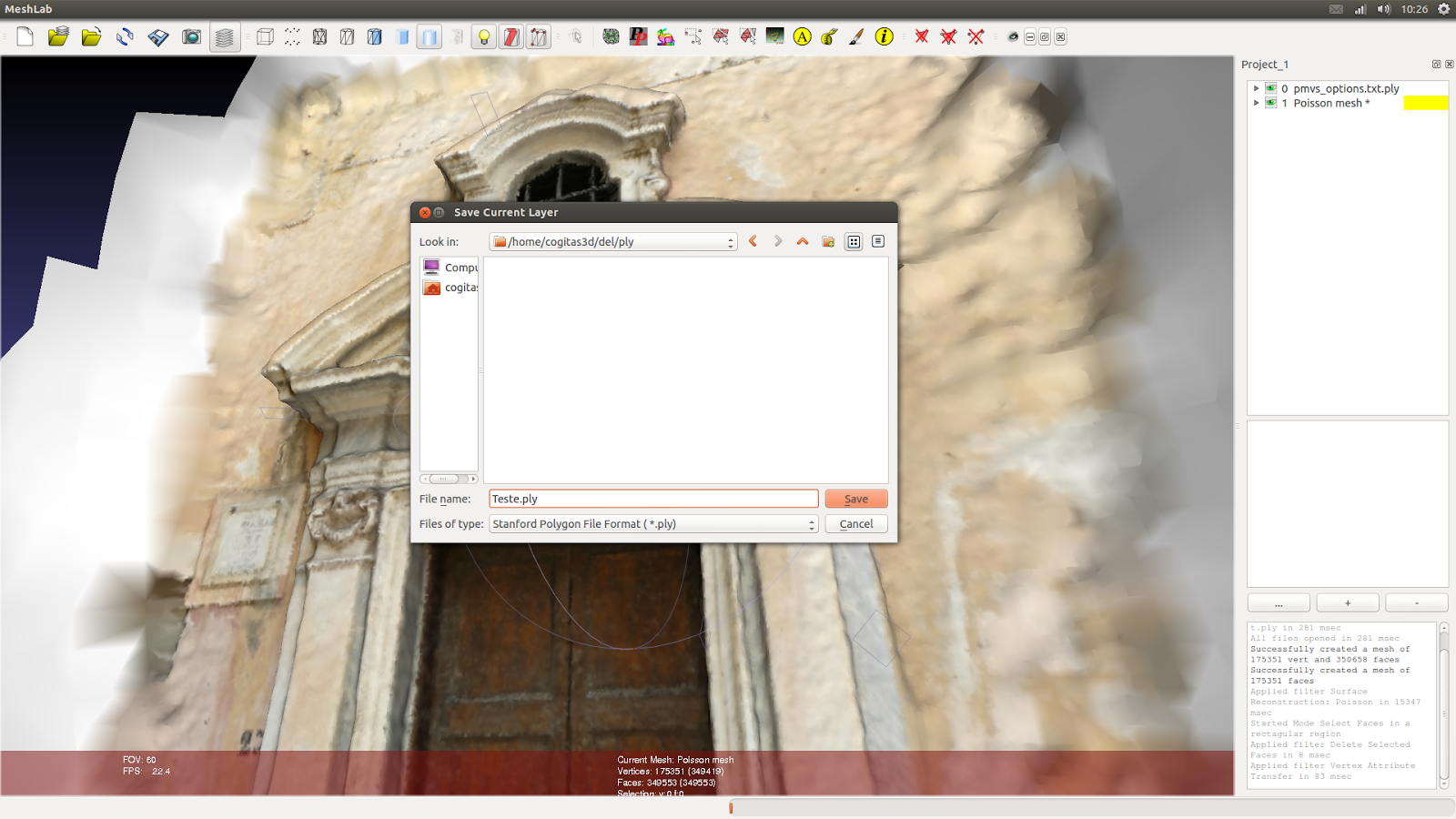
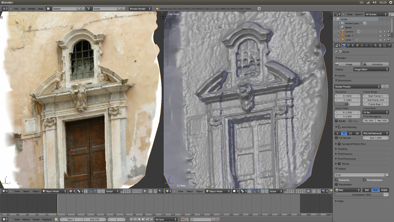
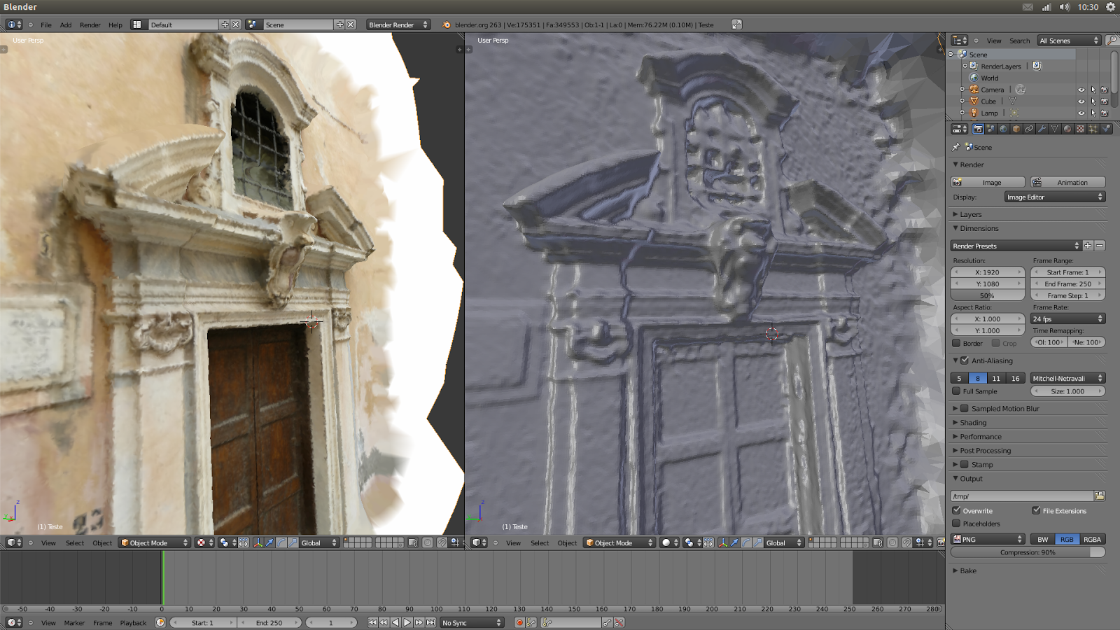
If you wanna send this mesh to other software like Blender, you can go to:
File -> Export Mesh As..
Choose a place to save the .PLY file.
If all is OK, the mesh will be imported on Blender (or other software) perfectly.
Other examples:
If you wanna you can download a sequence of pictures of Taung Child (anim. above) to make your own test here: