The devils boat

This year, thanks to Prof. Tiziano Camagna, we had the opportunity to prove our methodologies during a particular archaeological expedition, focused on the localization and documentation of the "devils boat". 

This strange wreck consists in a small boat built by the Italian soldiers, the "Alpini" of the battalion "Edolo" (nicknamed the "Adamello devils"), during the World War 1, near the mountain hut J. Payer (as reported by the book of Luciano Viazzi "I diavoli dell'Adamello"). 

The mission was a derivation of the project "La foresta sommersa del lago di Tovel: alla scoperta di nuove figure professionali e nuove tecnologie al servizio della ricerca” ("The submerged forest of lake Tovel: discovering new professions and new technologies at the service of scientific research"), a didactic program conceived by Prof. Camagna for the high school Liceo Scientifico B. Russell of Cles (Trentino - Italy).

As already mentioned, the target of the expedition has been the small boat currently lying on the bottom of lake Mandrone (Trentino - Italy), previously localized by Prof. Camagna and later photographed during an exploration in 2004. The lake is located at 2450 meters above see level. For this reason, before involving the students into such a difficult underwater project, a preliminary mission has been accomplished, in order to check the general conditions and perform some basic operations. This first mission was directed by Prof. Camagna and supported by the archaeologists of Arc-Team (Alessandro Bezzi, Luca Bezzi, for underwater documentation, and Rupert Gietl, for GNSS/GPS localization and boat support), by the explorers of the Nautica Mare team (Massimiliano Canossa and Nicola Boninsegna) and by the experts of Witlab (Emanuele Rocco, Andrea Saiani, Simone Nascivera and Daniel Perghem).
The primary target of the first mission (26 and 27 August 2016) has been the localization of the boat, since it was not known the exact place where the wreck was laying. Once the boat has been re-discovered, all the necessary operations to georeference the site have been performed, so that the team of divers could concentrate on the correct archaeological documentation of the boat. Additionally to the objectives mentioned above, the mission has been an occasion to test for the first time on a real operating scenario the ArcheoROV, the Open hardware ROV which has been developed by Arc-Team and WitLab.
Target 1 has been achieved in a fast and easy way during the second day of  mission (the first day was dedicated to the divers acclimation at 2450 meters a.s.l.), since the weather and environmental conditions were particularly good, so that the boat was visible from the lake shore. Target 2 has been reached positioning the GPS base station on a referenced point of the "Comitato Glaciologico Trentino" ("Galciological Committee of Trentino") and using the rover with an inflatable kayak to register some Control Points on the surface of the lake, connected through a reel with strategical points on the wreck. Target 3 has been completed collecting pictures for a post-mission 3D reconstruction through simple SfM techniques (already applied in underwater archaeology). The open source software used in post-processing are PPT and openMVG (for 3D reconstruction), MeshLab and CloudCompare (for mesh editing), MicMac (for the orthophoto) and QGIS (for archaeological drawing), all of them running on the (still) experimental new version of ArcheOS (Hypatia). Unlike what has been done in other projects, this time we preferred to recover original colours form underwater photos (to help SfM software in 3D reconstruction), using a series of command of the open source software suite Image Magick (soon I'll writ  a post about this operation). Once completed the primary targets, the spared time of the first expedition has been dedicated to secondary objectives: teting the ArcheoROV (as mentioned before) with positive feedbacks, and the 3D documentation of the landscape surrounding the lake (to improve the free LIDAR model of the area).
What could not be foreseen for the first mission was serendipity: before emerging from the lake, the divers of Nautica Mare team (Nicola Boninsegna and Massimiliano Canossa) found a tree on the bottom of the lake. From an archaeological point of view it has been soon clear that this could be an import discovery, as the surrounding landscape (periglacial grasslands) was without wood (which is almost 200 meters below). The technicians of Arc-Team geolocated the trunk with the GPS, in order to perform a sampling during the second mission.
For this reason, the second mission changed its priority an has been focused on the recovering of core samples by drilling the submerged tree. Further analysis (performed by Mauro Bernabei, CNR-ivalsa) demonstrated that the tree was a Pinus cembra L. with the last ring dated back to 2931 B.C. (4947 years old). Nevertheless, the expedition has maintained its educational purpose, teaching the students of the Liceo Russell the basics of underwater archaeology and performing with them some test on a low-cost sonar, in order to map part of the lake bottom.
All the operations performed during the two underwater missions are summarized in the slides below, which come from the lesson I gave to the student in order to complete our didactic task at the Liceo B. Russell.

Aknowledgements

Prof. Tiziano Camagna (Liceo Scientifico B. Russell), for organizing the missions

Massimiliano Canossa and Nicola Boninsegna (Nautica Mare Team), for the professional support and for discovering the tree

Mauro Bernabei and the CNR-ivalsa, for analizing and dating the wood samples

The Galazzini family (tenants of the refuge “Città di Trento”), for the logistic support

The wildlife park “Adamello-Brenta” and the Department for Cultural Heritage of Trento (Office of Archaeological Heritage) for close cooperation

Last but not least, Dott. Stefano Agosti, Prof. Giovanni Widmann and the students of Liceo B. Russel: Borghesi daniele, Torresani Isabel, Corazzolla Gianluca, Marinolli Davide, Gervasi Federico, Panizza Anna, Calliari Matteo, Gasperi Massimo, Slanzi Marco, Crotti Leonardo, Pontara Nicola, Stanchina Riccardo

Basic Principles of 3D Computer Graphics Applied to Health Sciences

Dear friends,

This post is an introductory material, created for our online and classroom course of "Basic Principles of 3D Computer Graphics Applied to Health Sciences". The training is the result of a partnership that began in 2014, together with the renowned Brazilian orthognathic surgeon, Dr. Everton da Rosa.

Initially the objective was to develop a surgical planning methodology using only free and freeware software. The work was successful and we decided to share the results with the orthognathic surgery community. As soon as we put the first contents related to the searches in our social media, the demand was great and it was not only limited to the professionals of the Dentistry, but extended to all the fields of the human health as well as veterinary.

In view of this demand, we decided to open the initial and theoretical contents of the topics that cover our course (which is pretty practical). In this way, those interested will be able to learn a little about the concepts involved in the training, while those in the area of ​​computer graphics will have at hand a material that will introduce them to the field of modeling and digitization in the health sciences.

In this first post we will cover the concepts related to 3D objects and scenes visualization.

We hope you enjoy it, good reading!

Chapter 1 - Scene Visualization

You already know much of what you need

Cicero Moraes
Arc-Team Brazil

Everton da Rosa
Hospital de Base, Brasília, Brazil

What does it take to learn how to work with 3D?

If you are a person who knows how to operate a computer and at least have already edited a text, the answer is, little.

When editing a text we use the keyboard to enter the information, that is, the words. The keyboard helps us with the shortcuts, for example the most popular CTRL + C and CTRL + V for copy and paste. Note that we do not use the system menu to trigger these commands for a very simple reason, it is much faster and more convenient to do them by the shortcut keys.

When writing a text we do not limit ourselves to writing a sentence or writing a page. Almost always we format the letters, leaving them in bold, setting them as a title or tilting them and importing images or graphics. These latter actions can also be called interoperability.

The name is complex, but the concept is simple. Interoperability is, roughly speaking, the ability of programs to exchange information with one another. That is, you take the photo from a camera, save it on the PC, maybe use an image editor to increase the contrast, then import that image into your document. Well, the image was created and edited elsewhere! This is interoperability! The same is true of a table, which can be made in a spreadsheet editor and later imported into the text editor.

This amount of knowledge is not trivial. We could say that you already have 75% of all the computational skills needed to work with 3D modeling.

Now, if you are one of those who play or have already played a first-person shooter game, you can be sure that you have 95% of everything you need to model in 3D.

How is this possible?

Very simple. In addition to all the knowledge surrounding most computer programs, as already mentioned, the player still develops other capabilities inherent in the field of 3D computer graphics.

When playing on these platforms it is necessary first of all to analyze the scene to which one is going to interact. After studying the field of action, the player moves around the scene and if someone appears on the line the chance of this individual to take a shot is quite large. This ability to move and interact in a 3D environment is the starting piece for working with a modeling and animation program.

 

Observation of the scene

When we get to an unknown location, the first thing we do is to observe. Imagine that you will take a course in a certain space. Hardly anyone "arrives rushed in’’ an environment. First of all we observe the scene, we make a general survey of the number of people and even study the escape routes in case of a very serious unforeseen event. Then we move through the studied scene, going to the place where we will wait for the beginning of the activities. In a third moment, we interact with the scenario, both using the course equipment such as notebook and pen, as well as talking to other students and / or teachers.

Notice that this event was marked by three phases:

1) Observation

2) Displacement

3) Interaction

In the virtual world of computer graphics the sequence is almost the same. The first part of the process consists in observing the scene, in having an idea of ​​what it is like. This command is known as orbit. That is, an observer orbit (Orbit) the scene watching it, as if it were an artificial satellite around the earth. It maintains a fixed distance and can see the scene from every possible angle.

But, not only orbiting man lives, one must approach to see the details of some specific point. For this we use the zoom commands, already well known to most computer operators. Besides zooming in and out (+ and - zooming) you also need to walk through the scenes or even move horizontally (a movement known as Pan).

A curious fact about these scene-observation commands is that they almost always focus on the mouse buttons. See the table below:

We have above the comparative of three programs that will be discussed later. The important thing now is to know that in the three basic zoom commands we see the direct involvement of the mouse. This makes it very clear that if you come across an open a 3D scene and use these combinations of commands, at least you will shift the viewer .

The phrase "move the observer" has been spelled out, so that you are aware of a situation. So far we are only dealing with observation commands. By the characteristic of its operation, it can very well be confused with the command of rotation of the object. As some would say, "Slow down. It's not quite that way. This is this, and that is that. ". It is very common for beginners in this area to be confused between one and the other.

To illustrate the difference between them, observe in the figure above the scene to the center (Original) that is the initial reference. On the left we observe the orbit command in action (Orbit). See that the grid element (in light gray) that is reference of what would be the floor of the scene accompanies the cube. This is because in fact the one who moves in the scene is the observer and not the elements. At the right side (Rotate) we see the grid in the same position as in the scene in the center, that is, the observer remained at the same point, except that the cube underwent rotation.

Why does this seem confusing?

In the real world, the one we live in, the observer is ... you. You use your eyes to see the space with all the three-dimensional depth that this natural binocular system offers. When we work with 3D modeling and animation software, your eyes become 3D View, that is, the working window where the scene is being presented.

In the real world, when we walk through a space, we have the ground to move. It is our reference. In a 3D scene usually this initial ground is represented by the grid that we saw in the example figure. It is always important to have a reference to work, otherwise it is almost impossible, especially for those who are starting, to do something on the computer.

Display Type

"Television makes you fatten".

Surely you have  already heard this phrase in some interview or even some acquainted or someone that had already been filmed and saw the result on the screen. In fact, it can happen that the person seems more robust than the "normal", but the answer is that, in fact, we are all more full-bodied than the structure that our eyes present to us when we look at ourselves in front of the mirror.

In order for you to have a clear idea of ​​what this means, you need to understand some simple concepts that involve viewing from an observer in a 3D modeling and animation program.

The observer in this case is represented by a camera.

Interestingly, one of the most used representations for the camera within a 3D scene is an icon of a pyramid. See the figure above, where three examples are presented. Both Blender 3D software and MeshLab have a pyramid icon to represent the camera in space. The simplest way to represent this structure can be a triangle, like the one on the right side (Icon).

All this is not for nothing. This representation holds in itself the basic principles of photography.

You may have heard of the pinhole camera(dark chamber). In a free translation it means photographic camera of hole. The operation of this mechanism is very simple, it is an archaic camera made with a small box or can. On one side it has a very thin hole and on the other side a photo paper is placed. The hole is covered by a dark adhesive tape until the photographer in question positions the camera in a point. Once the camera is positioned and still, the tape is removed and the film receives the external light for a while. Then the hole is again capped, the camera is transported to a studio and the film revealed, presenting the scene in negative. All simple and functional.

For us what matters is even a few small details. Imagine that we have an object to be photographed (A), the light coming from outside enters the camera through a hole made in the front (B) and projects the inverted image inside the box (C). Anything outside this capture area will be invisible (illustration on the right).

At that point we already have the answer of why the camera icons are similar in different programs. The pyramid represents the projection of the visible area of the camera. Notice that projection of the visible area is not the same as the ALL visible area, that is,  we have a small presentation of how the camera receives the external scene.

Anything outside this projection simply will not appear in the scene, as in the case of the above sphere, which is partially hidden.

But there's still one piece left in this puzzle, which is why we seem more robust to TV cameras.

Note the two figures above. Looking at each other, we can identify some characteristics that differentiate them. The image on the left seems to be a structure that is being squeezed, especially when we see the eyes, which seem to jump sideways. On the right, we have a structure that, in relation to another, seems to have the eyes more centered, the nose smaller, the mouth more open and a little more upwards, we see the ears showing and the upper part of the head is notoriously bigger.

Both structures have a lot of visual differences ... but they are all about the same 3D object!

The difference lies in the way the photographs were made. In this case, two different focal lengths were used. 

Above we see the two pinhole camera on top. The image on the left indicates the focal length value of 15 and on the right we see the focal length value of 50. On one side we see a more compact structure (15), where the background is very close to the front and on the other a more stretched structure, with a more closed catch angle (50).

But why in this case of 15 focal length, the ears do not appear in the scene?

The explanation is simple and can be approached geometrically. Note that in order to frame the structure in the photo it was necessary to bring it close enough to the light inlet. In doing so, the captured volume (BB) only picks up the front of the face (Visible), hiding the ears (Invisible). At the end, we have a limited projection (CC) that suffers from certain deformation, giving the impression of the eyes being slightly separated.

With the focal length of 50 the visible area of the face is wider. We can attest this to the projection of the visible region, as we have done previously.

In this example we chose to frame the structure very close to the camera capture limits and thus to highlight the capture differences. Thus we clearly see how a larger value of focal length implies in a wider capture of the photographed structure. A good example is that, with a value of 15, we see the lower tips of the ears very discreetly, in 35 the structures are already showing, at 50 the area is almost doubled, and at 100 we have an almost complete view of the ears. Note also that in 100, the marginal region of the eyes transverse the structure of the head and in orthogonal (Ortho) the marginal region of the eyes is aligned with the same structure.

But what is an orthogonal view?

For comprehension to be more complete, let us go by parts.

If we isolate the edges of all the views, align the eyebrows and base of the chin and put the superimposed forms, we will see at the end that the smaller the focal distance, the smaller the structural area visualized. Among all the forms that stand out the most is the orthogonal view. It simply has more area than all the others. We see this to the extreme right by attesting to the blue color appearing in the marginal regions of the overlap.

But, and orthogonal projection, how does it work?

The best example is the facade of a house. Above the left we have a vision with focal length 15 (Perspective) and right in orthogonal.

Analyzing the capture with focal length 15, we have the lines in blue, as usual, representing the boundary of the visible area (limit of the image generated) and in the other lines the projection of some key parts of the structure.

The orthogonal view in turn does not suffer from deformation of the focal length. It simply receives the structural information directly, generating a graph consistent with the measurements of the original, that is, it shows the house "as it is." The process is very reminiscent of the x-ray projection, which represents the x-ray structure without (or almost without) perspective deformation.

Looking at the images side by side, from another point of view, it is possible to attest a marked difference between them. The bottom and top of the side walls are parallel, but if you draw a line in each of these parts in perspective, that path will end up at an intersection that is known as the vanishing point (A and B). In the case of the orthogonal view, the lines are not found, because ... they are parallel! That is, we again see that the orthogonal projection respects the actual structure of the object.

So you mean that orthogonal view is always the best option?

No, it is not always the best option because it all depends on what you are doing. Take as an example the front views, discussed earlier. Even if the orthogonal view offers a larger capture area (D) if we compare the exclusive regions of the orthogonal (E) with the exclusive regions viewed by the focal length perspective 15 (F), we will attest that even covering a smaller area of pixels, The view with perspective deformation contemplated regions that were hidden in the orthogonal view.

Moraes & Salazar-Gamarra (2016)

That answers the question about whether or not people gain weight. The longer the focal length, the more robust the face looks. But this does not mean to fatten or not, but to actually show its structure, that is, the orthogonal image is the individual in his measurements more coherent with the real volumetry.

The interesting thing about this aspect is that it shows that the eyes deceive us, the image we see of people does not correspond to what they are actually structurally speaking. What we see in the mirror does not either.

Professional photographers, for example, are experts for how to exploit this reality and to extract the maximum quality in their works.

View 3D

Have you ever wondered why you have two eyes and not just one? Most of the time we forget that we have two eyes, because we see only one image when we observe things around us.  

Take this quick test.

Look for a small object to look at (A), which is about a meter away. Position the indicator (B) pointing up at 15cm from the front of the eyes (C), aligned with the nose.

When looking at the object you will see an object and two fingers.

When looking at the finger, you will see a finger and two objects.

If you observe with just one eye, you will attest that each has a distinct view of the scene.

This is a very simple way to test the limits of the binocular visualization system characteristic of humans. It is also very clear why classic painters close one eye by measuring the proportions of an object with the paint-brush in order to replicate it on the canvas (see the bibliography link for more details). If they used both eyes it just would not work!

You must be wondering how we can see only one image with both eyes. To understand this mechanism a little better, let's take 3D cinema as an example.

What happens if you look at a 3D movie screen without the polarized glasses?

Something like the figure above, a distortion well known to those who have already overdone alcoholic beverages. However, even though it seems the opposite, there is nothing wrong with this image.

When you put on the glasses, each lens receives information related to your eye. We then have two distinct images, such as when we blink to see with only one side. "

Let's reflect a little. If the blurred image enters through the glasses and becomes part of the scenery, transporting us into the movies to the point of being frightened by debris of explosions that seem to be projected onto us ... it may be that the information we receive from the world Be blurred with it. Except that, in the brain, somewhere "magical" happens that instead of showing this blur, the two images come together and form only one.

But why two pictures, why two eyes?

The answer lies precisely in the part of the debris of the explosion coming to us. If you watch the same scene with just one eye, the objects do not "jump" over you. This is because stereoscopic vision (with both eyes) gives you the power to perceive the depth of the environment. That is, the notion of space that we have is due to our binocular vision, without it, although we have notion of the environment because of the perspective, we will very much lose the ability to measure its volume.

Para que você entenda melhor a questão da profundidade da cena, veja a seguinte imagem.

To better understand the depth of the scene, see the following image.

If a group of individuals were asked which of the two objects is ahead of the scene, it is almost certain that most respondents would say that it is the object on the left.

However, not everything is what it seems. The object on the left is further away. This example illustrates how we can be deceived by monocular vision even though it is in perspective.

Would not it be easier for modeling and animation programs to support stereoscopic visualization?

In fact it could be, but the most popular programs still do not offer this possibility. In view of the popularization of virtual reality glasses and the convergence of graphic interfaces, the possibility of this niche has full support for the stereoscopic visualization in the production phase. However, this possibility is more a future projection than a present reality and the interfaces of today still count on many elements that go back decades.

It is for these and other reasons that we need the help of an orthogonal view when working on 3D software.

If on one hand we do not yet have affordable 3D visualization solutions with depth, on the other hand we have robust tools tested and approved for years and years of development. In 1963, for example, the Sketchpad graphic editor was developed at MIT. Since then the way of approaching 3D objects on a digital screen has not changed so much.

The most important of all, is that the technique works very well and with a little training you calmly adapt the methodology, to the point of forgetting that one day you had difficulties with that.

Almost all modeling programs, similar to Sketchpad, offer the possibility of dividing the workspace into four views: Perspective, Front, Right, and Top.

Even though it is not a perspective from which we have the notion of depth, and even the other views being a sort of "facade" of the scene, what we have in the end is a very clear idea of the structure of the scene and the positioning of the objects .

If, on the one hand, dividing the scene into four parts reduces the visual area of each view, on the other hand the specialist can choose to change those views in the total area of the monitor.

Over time, the user will specialize in changing the point of view using the shortcut keys, in order to complete the necessary information and not make mistakes in the composition of the scene.

A sample of the versatility of 3D orientation from orthogonal views is the exercise of the "hat in the little monkey" passed on to beginner students of three-dimensional modeling. This exercise involves asking the students to put a hat (cone) on the primitive Monkey. When trying to use only the perspective view the difficulties are many, because it is very difficult those who are starting to locate in a 3D scene. They are then taught how to use orthogonal views (front, right, top, etc.). The tendency is that the students position the "hat" taking only a view as a reference, in this case front (Front). Only, when they change their perspective view, the hat appears dislocated. When viewed from another point of view, such as right (Right), they realize that the object is far from where it should be. Over time the students "get the hang of it" and change the point of view when working with object positioning.

If we look at the graph of the axes that appear to the left of the figures, we see that in the case of Front we have the information of X and Z, but Y is missing (precisely the depth where the hat was lost) and in the case of Right we have Y and Z , But the X is

 missing. The secret is always to orbit the scene or to alternate the viewpoints, so as to have a clear notion of the structure of the scene, thus grounding its future interventions.

Conclusion

For now that’s it, we will soon return with more content addressing the basic principles of 3D graphics applied to health sciences. If you want to receive more news, point out some correction, suggestion or even better know the work of the professionals involved with the composition of this material, please send us a message or even, like the authors pages on Facebook:

3D designer Cícero Moraes's Page

Dr. Everton da Rosa's Page

We thank you for your attention and we leave a big hug here.

See you next time!

Low cost human face prosthesis with the aid of 3D printing

Dear friends,

It is with great honor and joy that I communicate my participation, for the first time in fact, in the preparation of a human facial prosthesis. I started my studies in early 2016 with Dr. Rodrigo Salazar, who materialized the prosthesis and was kind enough to invite me, as a 3D designer, to compose the group led by Dr. Luciano Dib. The team, made up of specialists from the Paulista University (UNIP) at São Paulo, University of Illinois at Chicago and Information Technology Center. This scanning is a basis for a digital preparation of the prosthesis made on Blender 3D software, with the help of the 3DCS addon developed by our team (myself, Dr. Everton da Rosa and Dalai Felinto). What we did with the innovative techniques of 3D modeling so as to optimize the quality of prototypes of prostheses, the merit is all of doctors Salazar, Dib and team.

Authors of rehabilitation:

Rodrigo Salazar

Cicero Moraes

Rose Mary Seelaus

Jorge Vicente Lopes da Silva

Crystianne Seignemartin

Joaquim Piras de Oliveira.

Luciano Dib.

Publisher and infographics:

Cicero Moraes

Photos:

Rodrigo Salazar

How the technique works

Based on: Salazar-Gamarra et al. Monoscopic photogrammetry to obtain 3D models by a mobile device: a method for making facial prostheses. Journal of Otolaryngology Head & Neck Surgery 2016;45:33

Infographics: Cicero Moraes

The first part of the process consists in photographing the patient in 5 different angles with 3 heights each angle, totaling 15 photos.

These photos can be made with a mobile phone, then they are sent to an online photogrammetry service (3D scanning per photo) called Autodesk® Recap360.

In about 20 minutes the server completes the calculations and returns a three-dimensional mesh corresponding to the patient's scanned face (first column on the left).

This face is mirrored in order to supply the missing structure, using the face complete as a parameter. Through a Boolean calculation the excesses of the mirrored part are excluded, resulting from the process a digital prosthesis that fits the missing region (second column on the left).

The digital prosthesis is sent to a 3D printer that materializes the piece. Then the structure is positioned on the patient to see if there is a fitting (third column on the left).

Once the structure has fit, a wax replica of the 3D print is generated. The purpose of this replica is to improve the marginal regions of docking and prepares the region that will receive the glass eye (fourth column on the left).

Finally a mold is generated from the replica in wax. This mold receives several layers of silicone. Each layer is pigmented to make colors compatible with the patient's skin. At the end of the process the prosthesis is obtained and can be adapted directly on the face of the patient (first column on the right).

A little of history

The doctors Prof. Dr. Luciano Dib, MSc. Rodrigo Salazar and MAMS. Rose Mary Seelaus are members of the Latin American Society of Buccomaxillofacial Rehabilitation. Among the activities developed by the society is the biannual event, where the members selected speakers who would speak at the event. In the April 2014 event, one of these invited speakers was MAMS. Rosemary Seelaus (anaplastologist), a specialist in facial prostheses for humans for almost 20 years.

At this event In early 2014, during one of the congresses organized by the association, Dr. Dib instigated Dr. Salazar to do a master's degree, of which he would be the advisor. Both were interested in the sophisticated techniques of Rose Mary Seelaus and intended to approach her in the studies, but they found a barrier, because at that time the prostheses were made with high operating costs, making it difficult to apply in Latin American public hospitals like Brazil.

The specialists then approached Dr. Seelaus, inquiring her whether it would be possible to assist them in adapting the technique to the Brazilian reality, reducing costs and, in the face of this, popularizing it to be used by the greatest number of Health professionals, thus benefiting those people who would not have access through the classical methodology, because its high cost.

Rodrigo Salazar, Rosemary Seelaus, Jorge Vicente Lopes da Silva e Luciano Dib at DT3D of CTI Renato Archer, Campinas-SP

Dr. Salazar began his master's studies in 2015. In March of that year, after preliminary studies on photogrammetry (3D digitalization by photos), via the online 123D Catch solution, the researchers sought the CTI Renato Archer (ProMED), to helping them to carry out the project to create a low-cost facial prosthesis.

During that time, CTI/ProMED not only supported the project with the necessary 3D printing (tests and final versions), but also helped in the training of the team members, through specific guidelines and necessary for the evolution of technology, always with the support from the head of the DT3D sector, Dr. Jorge Vicente Lopes da Silva.

In December of 2015 the article about the initial methodology was written and sent for publication (which occurred in May 2016).

The researchers were successful because the technique developed by them matched the classical technology in the results, but the cost has declined considerably.

Cicero Moraes and Rodrigo Salazar, Lima, Peru

Also at the end of the year, Dr. Salazar started the talks with me about the project and the possibilities of helping the development of the technique at a higher level using my know-how in computer graphics applied to the health sciences.

Because of the two full agendas, we spent some time communicating, but we resumed the dialogue in early 2016 and in February I began my studies in this field.

In a few months thanks to the versatility of the free software and the support of Dr. Salazar, Dr. Dib and CTI / ProMED, we were able to further develop the technique of facial scanning and prosthesis making.

Tests of human facial scanning in high resolution from photogrammetry. Moraes and Salazar-Gamarra (2016)

We did a series of tests, comparisons and discussions until we proceeded with the production of a real prosthesis. In the first half of December a patient received this piece and the procedure was successful, with an impressive result.

Now, after the help that I humbly proposed to offer and the help of the specialists in each phase, the quality of the prosthesis, according to the own team, has surpassed the methodology of high cost!

I am extremely honored to be a part of this project and to be able to help people with an accessible and robust technology, born of a team work and very, very study, which obviously has a lot to develop yet.

Happy of the society that will receive all the result of the successes. Whether through procedures that elevate self-esteem and contribute to a full life for those who have been victims of cancer, or for those who want to access and help improve the technology with us.

CHNT 2016: book of abstracts online!

Hi all,

this short post is just to notify that the book of abstracts of the 21st International Conference on Cultural Heritage and NEW Technologies (CHNT 21, 2016), which took place in Vienna (16-18 November), is now available online on the main website of the event.

This direct link takes you to the whole document, while, if you want to give a look to our contribution ("Digitizing the excavation. Toward a real-time documentation and analysis of the archaeological record"), you can find it here.

CHNT 2016 Book of Abstracts (cover)

Have a nice day!

Comparing 7 photogrammetry systems. Which is the best one?

by Cicero Moraes
3D Designer of Arc-Team.

When I explain to people that photogrammetry is a 3D scanning process from photographs, I always get a look of mistrust, as it seems too fantastic to be true. Just imagine, take several pictures of an object, send them to an algorithm and it returns a textured 3D model. Wow!

After presenting the model, the second question of the interested parties always orbits around the precision. What is the accuracy of a 3D scan per photo? The answer is: submillimetric. And again I am surprised by a look of mistrust. Fortunately, our team wrote a scientific paper about an experiment that showed an average deviation of 0.78 mm, that is, less than one millimeter compared to scans done with a laser scanner.

Just like the market for laser scanners, in photogrammetry we have numerous software options to proceed with the scans. They range from proprietary and closed solutions, to open and free. And precisely, in the face of this sort of programs and solutions, comes the third question, hitherto unanswered, at least officially:

Which photogrammetry software is the best?

This is more difficult to answer, because it depends a lot on the situation. But thinking about it and in the face of a lot of approaches I have taken over time, I decided to respond in the way I thought was broader and more just.

The skull of the Lord of Sipan

In July of 2016 I traveled to Lambayeque, Peru, where I stood face to face with the skull of the Lord of Sipan. In analyzing it I realized that it would be possible to reconstruct his face using the forensic facial reconstruction technique. The skull, however, was broken and deformed by the years of pressure it had suffered in its tomb, found complete in 1987, one of the greatest deeds of archeology led by Dr. Walter Alva.

To reconstruct a skull I took 120 photos with an Asus Zenphone 2 smartphone and with these photos I proceeded with the reconstruction works. Parallel to this process, professional photographer Raúl Martin, from the Marketing Department of Inca University Garcilaso de la Vega (sponsor of my trip) took 96 photos with a Canon EOS 60D camera. Of these, I selected 46 images to proceed with the experiment.

Specialist of the Ministry of Culture of Peru initiating the process of digitalization of the skull (in the center)

A day after the photographic survey, the Peruvian Ministry of Culture sent specialists in laser scanning to scan the skull of the Lord of Sipan, carrying a Leica ScanStation C10 equipment. The final cloud of points was sent 15 days later, that is, when I received the data from the laser scanner, all models surveyed by photogrammetry were ready.

We had to wait for this time, since the model raised by the equipment is the gold standard, that is, all the meshes raised by photogrammetry would be compared, one by one, with it.

Full points cloud imported into MeshLab after conversion done in CloudCompare

The cloud of points resulting from the scan were .LAS and .E57 files ... and I had never heard of them. I had to do a lot of research to find out how to open them on Linux using free software. The solution was to do it in CloudCompare, which offers the possibility of importing .E57 files. Then I exported the model as .PLY to be able to open in MeshLah and reconstruct the 3D mesh through the Poisson algorithm.

3D mesh reconstructed from a points cloud. Vertex Color (above) and surface with only one color (below).

As you noted above, the jaw and surface of the table where the pieces were placed were also scanned. The part related to the skull was isolated and cleaned for the experiment to be performed. I will not deal with these details here, since the scope is different. I have already written other materials explaining how to delete unimportant parts of a cloud of points / mesh.

For the scanning via photogrammetry, the chosen systems were:

1) OpenMVG (Open Multiple View Geometry library) + OpenMVS (Open Multi-View Stereo reconstruction library): The sparse cloud of points is calculated in OpenMVG and the dense cloud of points in OpenMVS.

2) OpenMVG + PMVS (Patch-based Multi-view Stereo Software): The sparse cloud of points is calculated in the OpenMVG and later the PMVS calculates the dense cloud of points.

3) MVE (Multi-View Environment): A complete photogrammetry system.

4) Agisoft® Photoscan: A complete and closed photogrammetry system.

5) Autodesk® Recap 360: A complete online photogrammetry system.

6) Autodesk ® 123D Catch: A complete online photogrammetry system.

7) PPT-GUI (Python Photogrammetry Toolbox with graphical user interface): The sparse cloud of points is generated by the Bundler and later the PMVS generates the dense cloud.

* Run on Linux under Wine (PlayOnLinux).

Above we have a table concentrating important aspects of each of the systems. In general, at least apparently there is not one system that stands out much more than the others.

Sparse cloud generation + dense cloud generation + 3D mesh + texture, inconsiderate time to upload photos and 3D mesh download (in the cases of 360 Recap and 123D Catch).

Alignment based on compatible points

Aligner skulls

All meshes were imported to Blender and aligned with laser scanning.

Above we see all the meshes side by side. We can see that some surfaces are so dense that we notice only the edges, as in the case of 3D scanning and OpenMVG + PMVS. Initially a very important information... the texture in the scanned meshes tend to deceive us in relation to the quality of the scan, so, in this experiment I decided to ignore the texture results and focus on the 3D surface. Therefore, I have exported all the original models in .STL format, which is known to have no texture information.

Looking closely, we will see that the result is consistent with the less dense result of subdivisions in the mesh. The ultimate goal of the scan, at least in my work, is to get a mesh that is consistent with the original object. If this mesh is simplified, since it is in harmony with the real volumetric aspect, it is even better, because, when fewer faces have a 3D mesh, the faster it will be to process it in the edition.

If we look at the file sizes (.STL exported without texture), which is a good comparison parameter, we will see that the mesh created in OpenMVG + OpenMVS, already clean, has 38.4 MB and Recap 360 only 5.1 MB!

After years of working with photogrammetry, I realized that the best thing to do when we come across a very dense mesh is to simplify it, so we can handle it quietly in real time. It is difficult to know if this is indeed the case, as it is a proprietary and closed solution, but I suppose both the Recap 360 and the 123D Catch generate complex meshes, but at the end of the process they simplify it considerably so they run on any hardware (PC and smartphones), preferably with WebGL support (interactive 3D in the internet browser).

Soon, we will return to discuss this situation involving the simplification of meshes, let us now compare them.

How 3D Mesh Comparison Works

Once all the skulls have been cleaned and aligned to the gold standard (laser scan) it is time to compare the meshes in the CloudCompare. But how does this 3D mesh comparison technology work?

To illustrate this, I created some didactic elements. Let's go to them.

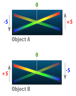
This didactic element deals with two planes with surfaces of thickness 0 (this is possible in 3D digital modeling) forming an X.

Then we have object A and object B. In the final portion of both sides the ends of the planes are distant in millimeters. Where there is an intersection the distance is, of course, zero mm.

When we compare the two meshes in the CloudCompare. They are pigmented with a color spectrum that goes from blue to red. The image above shows the two plans already pigmented, but we must remember that they are two distinct elements and the comparison is made in two moments, one in relation to the other.

Now we have a clearer idea of how it works. Basically what happens is the following, we set a distance limit, in this case 5mm. What is "out" try to be pigmented red, what is "in" tends to be pigmented with blue and what is at the intersection, ie on the same line, tends to be pigmented with green.

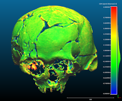
Now I will explain the approach taken in this experiment. See above we have an element with the central region that tends to zero and the ends that are set at +1 and -1mm. In the image does not appear, but the element we use to compare is a simple plane positioned at the center of the scene, right in the region of the base of the 3D bells, or those that are "facing upwards" when those that are "facing down" .

As I mentioned earlier, we have set the limit of comparison. Initially it was set at +2 and -2mm. What if we change this limit to +1 and -1mm? See that this was done in the image above, and the part that is out of bounds.

In order for these off-limits parts not to interfere with visualization, we can erase them.

Thus resulting in a mesh comprising only the interest part of the structure.

For those who understand a little more 3D digital modeling, it is clear that the comparison is made at the vertices rather than the faces. Because of this, we have a serrated edge.

Comparing Skulls

The comparison was made by FOTOGRAMETRIA vs. LASER SCANNING with limits of +1 and -1 mm. Everything outside that spectrum was erased.

OpenMVG+OpenMVS

OpenMVG+PMVS

Photoscan

MVE

Recap 360

123D Catch

PPT-GUI

By putting all the comparisons side by side, we see that there is a strong tendency towards zero, the seven photogrammetry systems are effectively compatible with laser scanning!

Let's now turn to the issue of file sizes. One thing that has always bothered me in the comparisons involving photogrammetry results was the accounting for the subdivisions generated by the algorithms that reconstruct the meshes. As I mentioned above, this does not make much sense, since in the case of the skull we can simplify the surface and yet it maintains the information necessary for the work of anthropological survey and forensic facial reconstruction.

In the face of this, I decided to level all the files, leaving them compatible in size and subdivision. To do this, I took as a base the smaller file that is generated by 123D Catch and used the MeshLab Quadratic Edge Collapse Detection filter set to 25000. This resulted in 7 STLs with 1.3 MB each.

With this leveling we now have a fair comparison between photogrammetry systems.

Above we can visualize the work steps. In the Original field are outlined the skulls initially aligned. Then in Compared we observe the skulls only with the areas of interest kept and finally, in Decimated we have the skulls leveled in size. For an unsuspecting reader it seems to be a single image placed side by side.

When we visualize the comparisons in "solid" we realize better how compatible they all are. Now, let's go to the conclusions.

Conclusion

The most obvious conclusion is that, overall, with the exception of MVE that showed less definition in the mesh, all photogrammetry systems had very similar visual results.

Does this mean that the MVE is inferior to the others?

No, quite the opposite. The MVE is a very robust and practical system. In another opportunity I will present its use in a case of making prosthesis with millimeter quality. In addition to this case he was also used in other projects of making prosthetics, a field that demands a lot of precision and it was successful. The case was even published on the official website of Darmstadt University, the institution that develops it.

What is the best system at all?

It is very difficult to answer this question, because it depends a lot on the user style.

What is the best system for beginners?

Undoubtedly, it's the Autodesk® Recap 360. This is an online platform that can be accessed from any operating system that has an Internet browser with WebGL support. I already tested directly on my smartphone and it worked. In the courses that I ministering about photogrammetry, I have used this solution more and more, because students tend to understand the process much faster than other options.

What is the best system for modeling and animation professionals?

I would indicate the Agisoft® Photoscan. It has a graphical interface that makes it possible, among other things, to create a mask in the region of interest of the photogrammetry, as well as allows to limit the area of calculation drastically reducing the processing time of the machine. In addition, it exports in the most varied formats, offering the possibility to show where the cameras were at the time they photographed the scene.

Which system do you like the most?

Well, personally I appreciate everyone in certain situations. My favorite today is the mixed OpenMVG + OpenMVS solution. Both are open source and can be accessed via the command line, allowing me to control a series of properties, adjusting the scanning to the present need, be it to reconstruct a face, a skull or any other piece. Although I really like this solution, it has some problems, such as the misalignment of the cameras in relation to the models when the sparse cloud scene is imported into Blender. To solve this I use the PPT-GUI, which generates the sparse cloud from the Bundler and the match, that is, the alignment of the cameras in relation to the cloud is perfect. Another problem with the OpenMVG + OpenMVS is that it eventually does not generate a full dense cloud, even if sparse displays all the cameras aligned. To solve this I use the PMVS which, although generating a mesh less dense than OpenMVS, ends up being very robust and works in almost all cases. Another problem with open source options is the need to compile programs. Everything works very well on my computers, but when I have to pass on the solutions to the students or those interested it becomes a big headache. For the end user what matters is to have a software in which on one side enter images and on the other leave a 3D model and this is offered by the proprietary solutions of objective mode. In addition, the licenses of the resulting models are clearer in these applications, I feel safer in the professional modeling field, using templates generated in Photoscan, for example. Technically, you pay the license and can generate templates at will, using them in your works. What looks more or less the same with Autodesk® solutions.

Acknowledgements

To the Inca University Garsilazo de la Vega for coordinating and sponsoring the project of facial reconstruction of the Lord of Sipán, responsible for taking me to Lima and Lambayeque in Peru. Many thanks to Dr. Eduardo Ugaz Burga and to Msc. Santiago Gonzáles for all the strength and support. I thank Dr. Walter Alva for his confidence in opening the doors of the Tumbas Reales de Sipán museum so that we could photograph the skull of the historical figure that bears his name. This thanks goes to the technical staff of the museum: Edgar Bracamonte Levano, Cesar Carrasco Benites, Rosendo Dominguez Ruíz, Julio Gutierrez Chapoñan, Jhonny Aldana Gonzáles, Armando Gil Castillo. I thank Dr. Everton da Rosa for supporting research, not only acquiring a license of Photoscan for it, but using the technology of photogrammetry in his orthognathic surgery plans. Dr. Paulo Miamoto for presenting brilliantly the results of this research during the XIII Brazilian Congress of Legal Dentistry and the II National Congress of Forensic Anthropology in Bahia. To Dr. Rodrigo Salazar for accepting me in his research group related to facial reconstruction of cancer victims, which caused me to open my eyes to many possibilities related to photogrammetry in the treatment of humans. To members of the Animal Avengers group, Roberto Fecchio, Rodrigo Rabello, Sergio Camargo and Matheus Rabello, for allowing solutions based on photogrammetry in their research. Dr. Marcos Paulo Salles Machado (IML RJ) and members of IGP-RS (SEPAI) Rosane Baldasso, Maiquel Santos and Coordinator Cleber Müller, for adopting the use of photogrammetry in Official Expertise. To you all, thank you!