by Cicero Moraes
3D Designer of Arc-Team.
When I explain to people that photogrammetry is a 3D scanning process from photographs, I always get a look of mistrust, as it seems too fantastic to be true. Just imagine, take several pictures of an object, send them to an algorithm and it returns a textured 3D model. Wow!
3D Designer of Arc-Team.
When I explain to people that photogrammetry is a 3D scanning process from photographs, I always get a look of mistrust, as it seems too fantastic to be true. Just imagine, take several pictures of an object, send them to an algorithm and it returns a textured 3D model. Wow!
After presenting the model, the second question of the interested parties always orbits around the precision. What is the accuracy of a 3D scan per photo? The answer is: submillimetric. And again I am surprised by a look of mistrust. Fortunately, our team wrote a scientific paper about an experiment that showed an average deviation of 0.78 mm, that is, less than one millimeter compared to scans done with a laser scanner.
Just like the market for laser scanners, in photogrammetry we have numerous software options to proceed with the scans. They range from proprietary and closed solutions, to open and free. And precisely, in the face of this sort of programs and solutions, comes the third question, hitherto unanswered, at least officially:
Which photogrammetry software is the best?
This is more difficult to answer, because it depends a lot on the situation. But thinking about it and in the face of a lot of approaches I have taken over time, I decided to respond in the way I thought was broader and more just.
The skull of the Lord of Sipan
In July of 2016 I traveled to Lambayeque, Peru, where I stood face to face with the skull of the Lord of Sipan. In analyzing it I realized that it would be possible to reconstruct his face using the forensic facial reconstruction technique. The skull, however, was broken and deformed by the years of pressure it had suffered in its tomb, found complete in 1987, one of the greatest deeds of archeology led by Dr. Walter Alva.

To reconstruct a skull I took 120 photos with an Asus Zenphone 2 smartphone and with these photos I proceeded with the reconstruction works. Parallel to this process, professional photographer Raúl Martin, from the Marketing Department of Inca University Garcilaso de la Vega (sponsor of my trip) took 96 photos with a Canon EOS 60D camera. Of these, I selected 46 images to proceed with the experiment.
 |
| Specialist of the Ministry of Culture of Peru initiating the process of digitalization of the skull (in the center) |
A day after the photographic survey, the Peruvian Ministry of Culture sent specialists in laser scanning to scan the skull of the Lord of Sipan, carrying a Leica ScanStation C10 equipment. The final cloud of points was sent 15 days later, that is, when I received the data from the laser scanner, all models surveyed by photogrammetry were ready.
We had to wait for this time, since the model raised by the equipment is the gold standard, that is, all the meshes raised by photogrammetry would be compared, one by one, with it.
 |
| Full points cloud imported into MeshLab after conversion done in CloudCompare |
The cloud of points resulting from the scan were .LAS and .E57 files ... and I had never heard of them. I had to do a lot of research to find out how to open them on Linux using free software. The solution was to do it in CloudCompare, which offers the possibility of importing .E57 files. Then I exported the model as .PLY to be able to open in MeshLah and reconstruct the 3D mesh through the Poisson algorithm.
 |
| 3D mesh reconstructed from a points cloud. Vertex Color (above) and surface with only one color (below). |
As you noted above, the jaw and surface of the table where the pieces were placed were also scanned. The part related to the skull was isolated and cleaned for the experiment to be performed. I will not deal with these details here, since the scope is different. I have already written other materials explaining how to delete unimportant parts of a cloud of points / mesh.
For the scanning via photogrammetry, the chosen systems were:
1) OpenMVG (Open Multiple View Geometry library) + OpenMVS (Open Multi-View Stereo reconstruction library): The sparse cloud of points is calculated in OpenMVG and the dense cloud of points in OpenMVS.
2) OpenMVG + PMVS (Patch-based Multi-view Stereo Software): The sparse cloud of points is calculated in the OpenMVG and later the PMVS calculates the dense cloud of points.
3) MVE (Multi-View Environment): A complete photogrammetry system.
4) Agisoft® Photoscan: A complete and closed photogrammetry system.
5) Autodesk® Recap 360: A complete online photogrammetry system.
6) Autodesk ® 123D Catch: A complete online photogrammetry system.
7) PPT-GUI (Python Photogrammetry Toolbox with graphical user interface): The sparse cloud of points is generated by the Bundler and later the PMVS generates the dense cloud.

* Run on Linux under Wine (PlayOnLinux).
Above we have a table concentrating important aspects of each of the systems. In general, at least apparently there is not one system that stands out much more than the others.

Sparse cloud generation + dense cloud generation + 3D mesh + texture, inconsiderate time to upload photos and 3D mesh download (in the cases of 360 Recap and 123D Catch).
 |
| Alignment based on compatible points |
 |
| Aligner skulls |
All meshes were imported to Blender and aligned with laser scanning.

Above we see all the meshes side by side. We can see that some surfaces are so dense that we notice only the edges, as in the case of 3D scanning and OpenMVG + PMVS. Initially a very important information... the texture in the scanned meshes tend to deceive us in relation to the quality of the scan, so, in this experiment I decided to ignore the texture results and focus on the 3D surface. Therefore, I have exported all the original models in .STL format, which is known to have no texture information.

Looking closely, we will see that the result is consistent with the less dense result of subdivisions in the mesh. The ultimate goal of the scan, at least in my work, is to get a mesh that is consistent with the original object. If this mesh is simplified, since it is in harmony with the real volumetric aspect, it is even better, because, when fewer faces have a 3D mesh, the faster it will be to process it in the edition.

If we look at the file sizes (.STL exported without texture), which is a good comparison parameter, we will see that the mesh created in OpenMVG + OpenMVS, already clean, has 38.4 MB and Recap 360 only 5.1 MB!
After years of working with photogrammetry, I realized that the best thing to do when we come across a very dense mesh is to simplify it, so we can handle it quietly in real time. It is difficult to know if this is indeed the case, as it is a proprietary and closed solution, but I suppose both the Recap 360 and the 123D Catch generate complex meshes, but at the end of the process they simplify it considerably so they run on any hardware (PC and smartphones), preferably with WebGL support (interactive 3D in the internet browser).
Soon, we will return to discuss this situation involving the simplification of meshes, let us now compare them.
How 3D Mesh Comparison Works
Once all the skulls have been cleaned and aligned to the gold standard (laser scan) it is time to compare the meshes in the CloudCompare. But how does this 3D mesh comparison technology work?
To illustrate this, I created some didactic elements. Let's go to them.

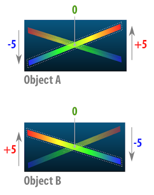
This didactic element deals with two planes with surfaces of thickness 0 (this is possible in 3D digital modeling) forming an X.

Then we have object A and object B. In the final portion of both sides the ends of the planes are distant in millimeters. Where there is an intersection the distance is, of course, zero mm.





Then we have object A and object B. In the final portion of both sides the ends of the planes are distant in millimeters. Where there is an intersection the distance is, of course, zero mm.

When we compare the two meshes in the CloudCompare. They are pigmented with a color spectrum that goes from blue to red. The image above shows the two plans already pigmented, but we must remember that they are two distinct elements and the comparison is made in two moments, one in relation to the other.

Now we have a clearer idea of how it works. Basically what happens is the following, we set a distance limit, in this case 5mm. What is "out" try to be pigmented red, what is "in" tends to be pigmented with blue and what is at the intersection, ie on the same line, tends to be pigmented with green.

Now I will explain the approach taken in this experiment. See above we have an element with the central region that tends to zero and the ends that are set at +1 and -1mm. In the image does not appear, but the element we use to compare is a simple plane positioned at the center of the scene, right in the region of the base of the 3D bells, or those that are "facing upwards" when those that are "facing down" .

As I mentioned earlier, we have set the limit of comparison. Initially it was set at +2 and -2mm. What if we change this limit to +1 and -1mm? See that this was done in the image above, and the part that is out of bounds.

In order for these off-limits parts not to interfere with visualization, we can erase them.

Thus resulting in a mesh comprising only the interest part of the structure.
For those who understand a little more 3D digital modeling, it is clear that the comparison is made at the vertices rather than the faces. Because of this, we have a serrated edge.
Comparing Skulls
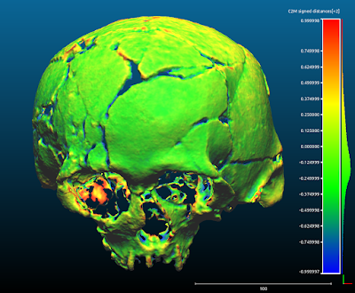
The comparison was made by FOTOGRAMETRIA vs. LASER SCANNING with limits of +1 and -1 mm. Everything outside that spectrum was erased.

OpenMVG+OpenMVS

OpenMVG+PMVS

Photoscan

MVE

Recap 360

123D Catch

PPT-GUI

By putting all the comparisons side by side, we see that there is a strong tendency towards zero, the seven photogrammetry systems are effectively compatible with laser scanning!

Let's now turn to the issue of file sizes. One thing that has always bothered me in the comparisons involving photogrammetry results was the accounting for the subdivisions generated by the algorithms that reconstruct the meshes. As I mentioned above, this does not make much sense, since in the case of the skull we can simplify the surface and yet it maintains the information necessary for the work of anthropological survey and forensic facial reconstruction.
In the face of this, I decided to level all the files, leaving them compatible in size and subdivision. To do this, I took as a base the smaller file that is generated by 123D Catch and used the MeshLab Quadratic Edge Collapse Detection filter set to 25000. This resulted in 7 STLs with 1.3 MB each.
With this leveling we now have a fair comparison between photogrammetry systems.

Above we can visualize the work steps. In the Original field are outlined the skulls initially aligned. Then in Compared we observe the skulls only with the areas of interest kept and finally, in Decimated we have the skulls leveled in size. For an unsuspecting reader it seems to be a single image placed side by side.

When we visualize the comparisons in "solid" we realize better how compatible they all are. Now, let's go to the conclusions.
Conclusion
The most obvious conclusion is that, overall, with the exception of MVE that showed less definition in the mesh, all photogrammetry systems had very similar visual results.
Does this mean that the MVE is inferior to the others?
No, quite the opposite. The MVE is a very robust and practical system. In another opportunity I will present its use in a case of making prosthesis with millimeter quality. In addition to this case he was also used in other projects of making prosthetics, a field that demands a lot of precision and it was successful. The case was even published on the official website of Darmstadt University, the institution that develops it.
What is the best system at all?
It is very difficult to answer this question, because it depends a lot on the user style.
What is the best system for beginners?
Undoubtedly, it's the Autodesk® Recap 360. This is an online platform that can be accessed from any operating system that has an Internet browser with WebGL support. I already tested directly on my smartphone and it worked. In the courses that I ministering about photogrammetry, I have used this solution more and more, because students tend to understand the process much faster than other options.
What is the best system for modeling and animation professionals?
I would indicate the Agisoft® Photoscan. It has a graphical interface that makes it possible, among other things, to create a mask in the region of interest of the photogrammetry, as well as allows to limit the area of calculation drastically reducing the processing time of the machine. In addition, it exports in the most varied formats, offering the possibility to show where the cameras were at the time they photographed the scene.
Which system do you like the most?
Well, personally I appreciate everyone in certain situations. My favorite today is the mixed OpenMVG + OpenMVS solution. Both are open source and can be accessed via the command line, allowing me to control a series of properties, adjusting the scanning to the present need, be it to reconstruct a face, a skull or any other piece. Although I really like this solution, it has some problems, such as the misalignment of the cameras in relation to the models when the sparse cloud scene is imported into Blender. To solve this I use the PPT-GUI, which generates the sparse cloud from the Bundler and the match, that is, the alignment of the cameras in relation to the cloud is perfect. Another problem with the OpenMVG + OpenMVS is that it eventually does not generate a full dense cloud, even if sparse displays all the cameras aligned. To solve this I use the PMVS which, although generating a mesh less dense than OpenMVS, ends up being very robust and works in almost all cases. Another problem with open source options is the need to compile programs. Everything works very well on my computers, but when I have to pass on the solutions to the students or those interested it becomes a big headache. For the end user what matters is to have a software in which on one side enter images and on the other leave a 3D model and this is offered by the proprietary solutions of objective mode. In addition, the licenses of the resulting models are clearer in these applications, I feel safer in the professional modeling field, using templates generated in Photoscan, for example. Technically, you pay the license and can generate templates at will, using them in your works. What looks more or less the same with Autodesk® solutions.
Acknowledgements
To the Inca University Garsilazo de la Vega for coordinating and sponsoring the project of facial reconstruction of the Lord of Sipán, responsible for taking me to Lima and Lambayeque in Peru. Many thanks to Dr. Eduardo Ugaz Burga and to Msc. Santiago Gonzáles for all the strength and support. I thank Dr. Walter Alva for his confidence in opening the doors of the Tumbas Reales de Sipán museum so that we could photograph the skull of the historical figure that bears his name. This thanks goes to the technical staff of the museum: Edgar Bracamonte Levano, Cesar Carrasco Benites, Rosendo Dominguez Ruíz, Julio Gutierrez Chapoñan, Jhonny Aldana Gonzáles, Armando Gil Castillo. I thank Dr. Everton da Rosa for supporting research, not only acquiring a license of Photoscan for it, but using the technology of photogrammetry in his orthognathic surgery plans. Dr. Paulo Miamoto for presenting brilliantly the results of this research during the XIII Brazilian Congress of Legal Dentistry and the II National Congress of Forensic Anthropology in Bahia. To Dr. Rodrigo Salazar for accepting me in his research group related to facial reconstruction of cancer victims, which caused me to open my eyes to many possibilities related to photogrammetry in the treatment of humans. To members of the Animal Avengers group, Roberto Fecchio, Rodrigo Rabello, Sergio Camargo and Matheus Rabello, for allowing solutions based on photogrammetry in their research. Dr. Marcos Paulo Salles Machado (IML RJ) and members of IGP-RS (SEPAI) Rosane Baldasso, Maiquel Santos and Coordinator Cleber Müller, for adopting the use of photogrammetry in Official Expertise. To you all, thank you!